ESE446: Robotics Dynamics and Control Final Project
� Adith Jagadish Boloor
Objective:� The objective of the project is to
gain understanding of various robot manipulator design tools and
characteristics.� Through the use of an
example we want to demonstrate the understanding of the Jacobian, robot
dynamics, trajectory, and manipulator control.�
The example to be used will be the 3R planar robot describe in the
figures illustrated below.
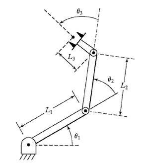
Figure 1: 3R Planar Robot
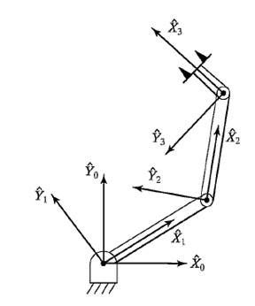
Figure 2: Frame layout for 3R Planar Robot
Task-1: Robot Simulation
Table 1: DH Link table for 3R Planar Robot
|
|
|
|
|
|
|
|
|
|
|
1 |
0 |
0 |
0 |
|
1 |
0 |
|
|
2 |
0 |
|
0 |
|
1 |
0 |
|
|
3 |
0 |
|
0 |
|
1 |
0 |
|
|
4 |
0 |
|
0 |
0 |
1 |
0 |
The Denavit�Hartenberg (DH)
parameters shown in table one is one way we can go about describing the
kinematics (position) of the robot arm. The parameters are described as
follows:
�
![]() ��
angle about the common normal, from the previous z-axis to the new z-axis
��
angle about the common normal, from the previous z-axis to the new z-axis
�
![]() ��
length of the common normal (in this case, the length of each non-prismatic
link)
��
length of the common normal (in this case, the length of each non-prismatic
link)
�
d
- �offset along previous z-axis to the common normal
�
![]() ��
angle about the previous z-axis from the previous x-axis to the new x-axis
��
angle about the previous z-axis from the previous x-axis to the new x-axis
The
transformation matrix is given by:
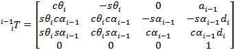
Note that the �s� denotes sine and �c� denotes cosine. The
transformation matrix is a mathematical representation of the pose for a
particular link (i) of a robot, with respect to the
previous link (i-1). The 3x3 sub-matrix of the transformation matrix is called
the rotational matrix:
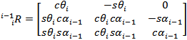
The rotational matrix
is a mathematical representation of the angle of the link with respect to the
previous link.
The 4th
column (neglecting the 4th row) of the transformation matrix is the
position vector as shown below:
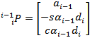
The position vector is
a mathematical representation of the position of the link with respect to the
previous link.
Using the DH matrix,
and the generalized formula for the transformation matrix shown above, the
transformation matrices can be calculated for each link. Note that zero is the
base �link�.
The most important
property of transformation matrices is that the pose of a link with respect to
the base can be calculated with ease using matrix multiplication as follows:
![]()
The same
method can be used to calculate the rotation matrices
T1 (Task-1) Derive dynamic equation
for manipulator.
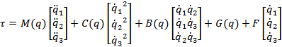
The dynamic
equation for any robot is given by the following equation which governs the
torque applied at the actuators and the external forces applied to the
manipulators, which is got from the Lagrangian, which
simply applies the conversation of energy principle.
�
![]() ��
tau vector (forces applied at the actuators)
��
tau vector (forces applied at the actuators)
�
![]() ��
mass matrix (mass distribution as a function of manipulator pose)
��
mass matrix (mass distribution as a function of manipulator pose)
�
![]() ��
centrifugal matrix
��
centrifugal matrix
�
![]() ��
Coriolis matrix
��
Coriolis matrix
�
![]() � gravitational force vector
� gravitational force vector
�
![]() � kinetic frictional force coefficients
� kinetic frictional force coefficients
�
![]() ��
generalized position of a joint
��
generalized position of a joint
�
![]() ��
angular velocity of joint i
��
angular velocity of joint i
�
![]() �-�
angular acceleration of joint i
�-�
angular acceleration of joint i
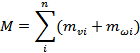
The
Mass Matrix:
To calculate the mass
matrix, we must first calculate the velocity and angular velocity Jacobians of each joint. In simple words, a Jacobian is a matrix whose elements show how each joint�s
spatial properties change with each other.
The velocity Jacobian is given by:
![]()
The q�s represent the
angular position of each respective link. ![]() �is the position vector of the center of mass for each link.
Note that each Jv will be a
3x3 matrix. This is given by:
�is the position vector of the center of mass for each link.
Note that each Jv will be a
3x3 matrix. This is given by:
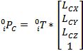
Where ![]() �is
the center of mass of that link in its zero (q1, q2 q3 = 0) position. In our
case, the center of mass vector looked like the following for each link.
�is
the center of mass of that link in its zero (q1, q2 q3 = 0) position. In our
case, the center of mass vector looked like the following for each link.

Where ![]() �is
the length of the i link. This assumes that the mass
is uniformly distributed along the links.
�is
the length of the i link. This assumes that the mass
is uniformly distributed along the links.
The angular Jacobian
is given by:
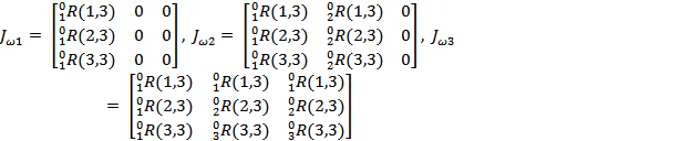
Here (i,3) etc., refers to the i�th
element of the third column of the rotation matrix. We use this because the
third column of the rotational matrix holds the angular information for that
link.
To represent the mass distribution
relating to the angular velocity, we also need the inertial properties of the
robot. The inertial matrix (also called Intertial
tensor) for each joint is given by:
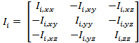
![]() �represents the moment of inertia about the x axis for each
link, and same goes for y and z.
�represents the moment of inertia about the x axis for each
link, and same goes for y and z. ![]() �represents the product of inertia between the
respective axes. Since our robot is a planar robot in the x and y coordinate
frame, we will have only
�represents the product of inertia between the
respective axes. Since our robot is a planar robot in the x and y coordinate
frame, we will have only ![]() . The other moments will be zero.
. The other moments will be zero.
Now to calculate the mass distribution
with respect to velocity and angular velocity for each link, we have:
![]()
![]()
The overall mass matrix is given by:
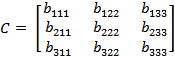
The
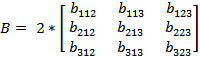
Centrifugal matrix (C) and Coriolis (B) matrix:
Like their name state, the
centrifugal matrix represents the centrifugal forces, and the Coriolis matrix represents the Coriolis
force experienced by the system.
The centrifugal matrix for a 3 link
RRR robot is given by:
And the Coriolis
matrix is given by:
Where, ![]() �(known as Christoffel Symbols) is given by:
�(known as Christoffel Symbols) is given by:
![]()
And
![]()
Where ![]() �is
the ij element of each matrix. Fun.
�is
the ij element of each matrix. Fun.
The gravity matrix:
The gravity matrix shows the forces
experienced by the robot in the negative y-direction (because of acceleration
due to gravity).
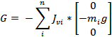
�
![]() ��
velocity Jacobian
��
velocity Jacobian
�
![]() - mass of each link
- mass of each link
�
![]() ��
acceleration due to gravity (+9.81m/s2)
��
acceleration due to gravity (+9.81m/s2)
The
Friction vector:
Ideally we would be
using both static and dynamic (kinetic) friction. But to keep it simple, we
will be using only dynamic friction, because we are more interested in what
happens to the robot during motion. Note that friction is very important in the
simulation of this robot. Because without it, there is no resistance for each
joint and they will behave sporadically.

Where ![]() �is
the coefficient of dynamic friction of each link.
�is
the coefficient of dynamic friction of each link.
Tau
vector:
After calculating all the vectors and
matrices, we can calculate the tau vector that comprises the forces at each
joint. Why do we call it tau instead of force? Who knows?
Just to recap, the formula is:
�
T1. Solve equations for acceleration and use these to create
state-space simulator.
We simply use the state space
equation mentioned previously to solve for the accelerations of each joint.
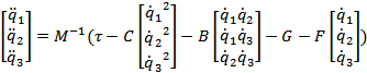
Check attachment (vectors_qpp_tau.txt)
for all the matrices and acceleration solutions.
T1. Use robot manipulator initial angles of 10, 20, and 30 degrees
respectively.
DONE.
T1. Use individual link lengths of 4,
3, and 2 meters respectively. DONE
T1. Use individual link masses of 20,
15, and 10 kg respectively. DONE
T1. Use a-axis inertial values of
0.5, 0.2, and 0.1 kg-m2 respectively. DONE
T1. Demonstrate dynamics of the robot
through simulation.
The Simulink
model looks like the following for T1:
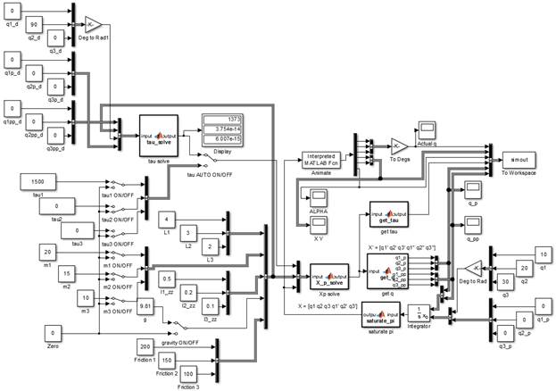
Figure 3: Simulink Model for Task1
Notice that
all parameters are changeable. The scopes can be used to check how each parameter
changes with the robot animation. On the right side of the image you can see
that the initial angles are set as 10, 20 and 30 degrees respectively.
1. No actuator torque, no gravity
Figure 4: Simulation - [tau1, tau2, tau3] = [0, 0, 0]; g = 0
The arm
stays still because there are no internal or external forces acting on it.
Created gif
using: https://ezgif.com/video-to-gif/
Converted avi to mp4 using: http://convert-video-online.com/
2. No actuator torque, with gravity
Figure 5: Simulation - [tau1, tau2, tau3] = [0, 0, 0]; g =
9.81m/s2
Here the arm
falls downwards, and oscillates about negative 0 in the y direction because
gravity is the force acting on it, which is in the negative y direction.
3. Joint-1 actuator torque in order to
provide equilibrium, with gravity
Figure 6: Simulation - [tau1, tau2, tau3] = [1845, 0, 0] N; g
= 9.81 m/s2
The tau
values for the joints are:
�
Joint
1 � 1845 N
�
Joint
2 � 0 N
�
Joint
3-� 0 N
The force
chosen at joint 1 is based on trying to establish equilibrium for the links at
10, 20 and 30 degrees respectively. The taus were
calculated using the Lagrangian equation derived
before, setting the velocities and accelerations to zero. Observe that just for
a brief second, link 1 stays at 10 degrees before the motion of other links
make the robot become unstable. This is because we are attempting to balance
the robot with a constant torque in an open-loop control method.
4. Joint-1 and Joint-2 actuator torque
in order to provide equilibrium, with gravity
Figure 7: Simulation - [tau1, tau2, tau3] = [1845, 495.1, 0]
N; g = 9.81 m/s2
The tau values
for the joints are:
�
Joint
1 - 1845 N
�
Joint
2 - 495.1 N
�
Joint
3-� 0 N
The forces
chosen at joint 1 and 2, are based on trying to establish equilibrium for the
links at 10, 20 and 30 degrees respectively. Observe that just for a brief
second, links 1 and 2 stay at 10 and 20 degrees respectively before the motion
of other links make the robot become unstable. Also note that this time the
robot stays in equilibrium a bit longer than while we used torque at only one
joint. Again this is because we are attempting to balance the robot with a
constant torque in an open-loop control method.
5. Joint-1,
Joint-2, and Joint-3 actuator torque in order to provide equilibrium, with
gravity
Figure 8: Simulation - [tau1, tau2, tau3] = [1845, 495.1,
49.05] N; g = 9.81 m/s2
The tau
values for the joints are:
�
Joint
1 - 1845 N
�
Joint
2 - 495.1 N
�
Joint
3-� 49.05 N
The forces
chosen at joint 1, 2 and 3, are based on trying to establish equilibrium for
the links at 10, 20 and 30 degrees respectively. Observe that this time, the
robot stays in equilibrium a lot longer. However it becomes unstable because of
tiny changes in position of the links (most like caused because of the forces�
precision). Again this is because we are attempting to balance the robot with
using open-loop control.
T1. All simulations should present
graphs of x,y, and alpha
end-effector positions vs. time.
Did one
better. Added tau, q, q� and q�� vs time graphs as
well
T1. Include any other graphs, gif�s,
etc. which you deem necessary to describe the demonstration. DONE
Task-2 Robot simulation � with
control partitioning
T2 (Task 2) Design a closed loop
system by partitioning the robot dynamics into model-based and servo-based
dynamics.
For task 2,
we are incorporating a position and velocity controlled closed loop.
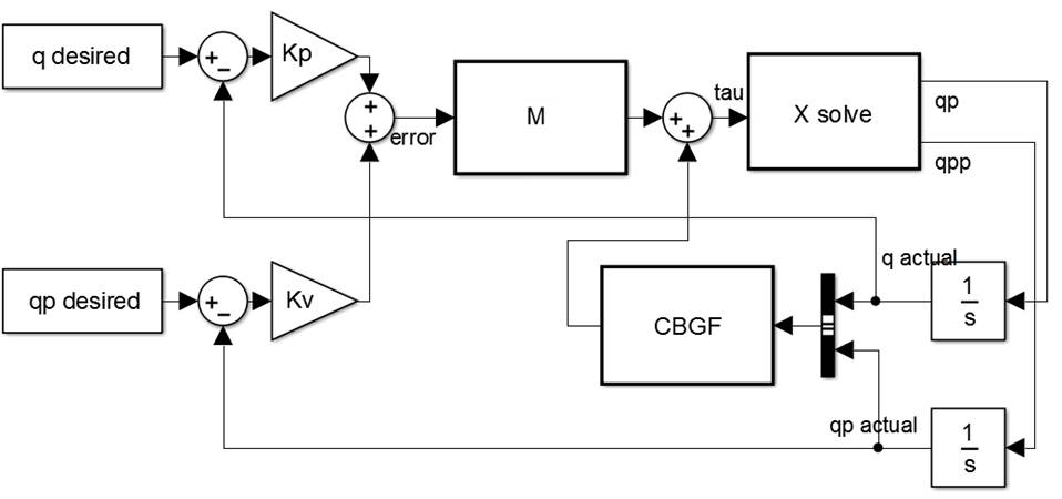
Figure 9: Closed loop control
Figure 9
shows us how the desired and actual position and velocity are being multiplied
by their respective gains (Kp
and Kv), and summed up. Kp and Kv are essentially
the weightage we give for these error signals. This gives us the overall error
in q. This is fed into the mass matrix (M) and summed up with the centrifugal
(C), Coriolis (B), gravity (G) and friction (F)
matrices/vectors to give us the forces (tau). Using the tau, we can solve for
the accelerations (qpp) using the Lagrangian
equation mentioned earlier. The output of this being the acceleration and the
velocity (qp) go through an
integrator to get the actual velocity and position of the robot. These values
are used for the CBGF calculations and for subtracting them from the actual
position and velocity respectively. The control loop tries to get the error to
zero. The Kp tells us how
fast it will try to decrease the error, while the Kv
helps damped the motion as the error is decreased. A good place to start Kp is at 1, and increase it. Kv is typically twice the square root of Kp.
T2. Simulate the system by setting
the initial joint angles to 10, 20, and 30 degrees respectively. Explain what
happens during the simulation.
The Simulink
model for task 2 is as follows:
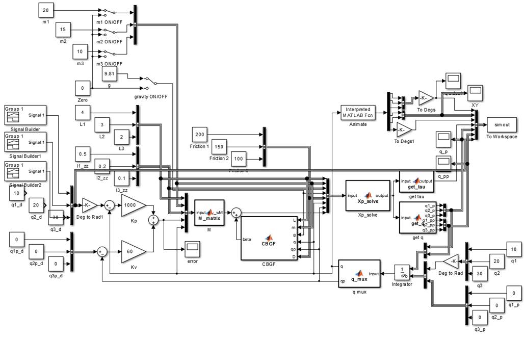
Figure 10: Task 2 Simulink Model
The
simulation will be explained in the subsequent subsections.
T2. Add joint-position control by
adding an input vector which represents the joint desired positions. DONE
T2. Simulate the system with the
above initial angles and appropriate input command angles. DONE
T2. One joint at a time, apply a step
input change to the command angle. Monitor the response of the system by
examining the error signal.
A simple
demo was done incorporating the above closed loop control with Kp = 10 and Kv
= 6. Several desired positions (or command angles) were used to check the
effectiveness of the control as you can see in the following animation.
Figure 11: Animation - Kp
= 10 Kv = 6 for different command angles
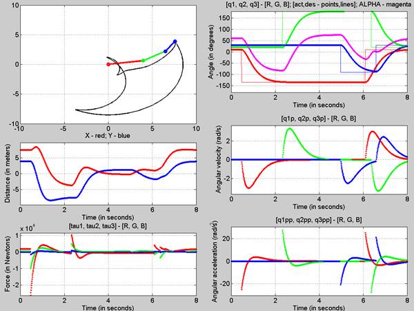
Figure 12: Final Pose - Kp
= 10, Kv = 6
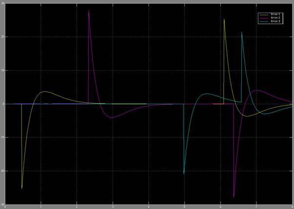
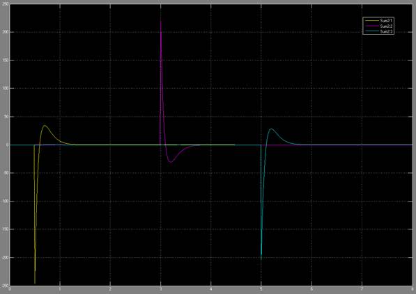
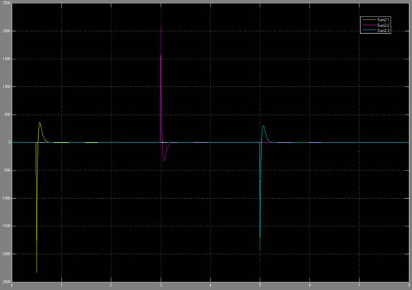
Figure 13: Error signal through the changes in command angle
Figure 11
shows the animation of the robot as it goes to the input desired angles. You
can see from the q subplot (figure 12) how the robot moves to those angles. The
response looks like a first order system. In figure 13, you can see the error
signals, which we try to get to zero using the closed loop control. We can see
that there is some over shoot for all the joints. This can be mitigated by
choosing different kp and kv values.
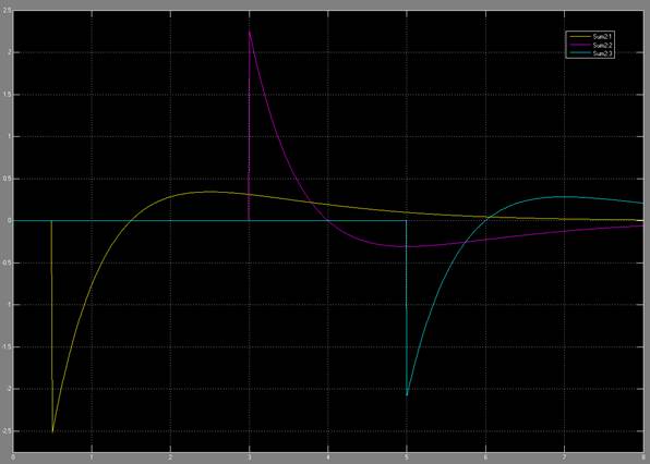
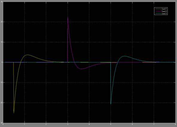
T2. Experiment with various Kp gains (such as 1, 10, 100,
etc.) and explain the results.
To run the
same experiments for different gains, a signal builder was used that set the
command angle for q1 to -135 degs at 0.5 seconds, q2
to 150 degs at 3 seconds and q3 to -90 degrees at 5
seconds each time.
Kp = 1; Kv =
1
 �
� �
�
Kp = 1; Kv =
2
 �
�
Kp = 10; Kv =
6
 �
�
Kp = 100; Kv
= 20
 �
�
Kp = 1000; Kv
= 60
 �
�
The higher
the Kp value, the faster the
response of the system is, i.e., the higher the gains, the faster the errors
get driven to zero. Since this is a simulated system, we have no repercussions
of using higher and higher gains, however in a real system the higher the
gains, the more energy (in terms of voltage) you would need to supply.
Additionally in a real system, using very high gains could damage components
like gears and the motor.
T2. How does the rise time change? Talked about in the next subsection.
T2. Can you set the gain to give
overshoot?
The
following table is made from the data above for q1 to give us a better
understanding of how rise time and overshoot varies with Kp and Kv.
Table 2: Kp,
Kv vs Rise time and
Overshoot
|
Kp |
Kv |
Rise time (s) |
Overshoot > 5%? |
|
1 |
1 |
2.5 |
YES |
|
1 |
2 |
5.5 |
NO |
|
10 |
6 |
2 |
NO |
|
100 |
20 |
1 |
NO |
|
1000 |
60 |
0.25 |
NO |
We can
observe that the rise time decreases with increasing Kp,
provided the Kv matches it (~2xsqrt(Kp)). Gains can be set to create overshoot. A Kp with the Kv lesser than 2sqrt(Kp) will create overshoot. Kv helps to dampen the system, hence it would make sense
that if it is too small, the system would oscillate.
T2. Does the system need different Kp values for each joint?
As can be
observed from the system above, you do not necessarily need different Kp values for each joint to get a
fast response without overshoot. However, if you wanted the responses for each
joint to be different, they would need different gains.
T2. Does the step response look like
a second order system?
No, as long as the Kp and Kv values match each other (Kv ~ 2sqrt(Kp)), the system looks like
a first order system. However, if the Kv is too low,
the system could behave as a second order system.
Task-3: Robot simulation � path
trajectory
Most
industrial robot paths are programmed by teaching desired points along the
path. This is done by using the teach pendant to maneuver to some desired point
and orientation and then capturing the joints coordinate values. Given these
joint coordinates and some desired time line we can create a reasonable
trajectory through these points.
Given: The
following timeline data
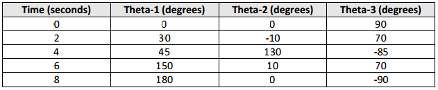
T3. (Task 3) Create a spline fit
curve through each set of points for each joint. Make sure the starting and
ending slopes of the trajectory (joint velocity) are zero. (Use the spline function
in MATLab).
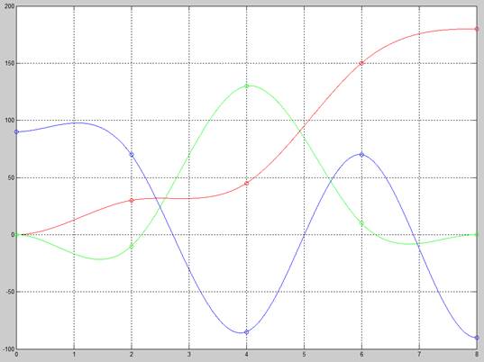
Figure 14: Cubic splines for q1, q2 and q3 (R, G, B)
Write a function to feed the three
trajectory curves to your RRR robot simulator. DONE
Set initial angles of system to match
those at time zero and simulate the path for 8 seconds. DONE
The
following trajectory animations use Kp
= 1000 and Kv = 60
Figure 15: Trajectory follower using Signal Builder
Figure 15
was the result of using a signal builder. The signal for q1 looked like the
following:
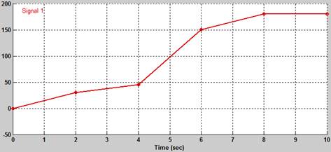
Figure 16: Signal Builder for q1
The
following figure shows the animation using the spline function in MATLAB.
Figure 17: Animation with MATLAB's spline function
We can
observe that the simulation using the MATLAB�s function is smoother, i.e., have
steadier position slopes. We can also see that the velocity profiles are not as
abrupt as the one using the signal builder.
Does the simulation make it to the
end?
Yes
Does the value of the selected gains
(Kp and Kv)
change the simulation?
Ofcourse.
The following animation has a Kp
of 1 and a Kv of 2:
Figure 18: Trajectory follower with Kp=1 and Kv
= 2
We notice
that there is a large error between the desired and actual joint angles. This
is because of the small Kp.
Does the actual path follow the
designed trajectory?
It does not exactly follow the desired q angles between the
set points at 2, 4, 6 and 8 seconds. However, Kp and Kv can be tuned to
achieve it.
Bonus
Figure 19: My attempt at writing ESE with the robot